dynamical systems: act2020 blog post-er
I messed up with the title of this paper, it sounds way too crackpotty. I’ll explain what I mean in this 5-minute read, with lots of illustrations, building on a running example.
The Allee Effect is a phenomenon in population dynamics where a the population of a speciees tends to die out if it falls below a critical point, and above the critical point the population enjoys (logistic) growth. Say we have a population of Things (T). In the plot of the rate-of-change-over-time-of-T against T, the Allee effect looks something like this:
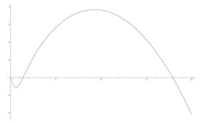
Typically, the Allee effect is modelled by a cubic first-order ordinary differential equation, with roots at 0, the critical population point, and the ‘carrying capacity’ of the ecosystem. I had an intellectual problem with this descriptivist approach, so I tried to come up with something better.
A. the problem
Say you gathered some data on the population T, observed an Allee Effect, and then fit the coefficients of the cubic F-O ODE to obtain a model for the dynamical system of the population. Now somebody asks:
“Say doc, what happens if we make the things breed faster?”
“What if we decreased predation of Things?”
“Would we still see the Allee Effect?”
…and you’re stuck. There’s just no way to model the effect of interventions without something underneath the dynamical system that has enough structure for the interventions to talk to. Even if you had a good idea what the underlying processes governing the dynamics are, how does that reflect in the coefficients of a F-O ODE?
B. the solution
TL;DR: Use Law of Mass Action to get F-O ODEs from Petri Nets that model your “causal-mechanistic” assumptions, with a free coefficient for each transition in the net. Then you can fit those coefficients to agree with empirical data to obtain models, and then you can manipulate those coefficients to model interventions.
So having a “causal-mechanistic” account of the dynamical system is a necessary startup cost for this approach, but the bonus is that you can falsify those accounts: once you have a fitted model for a dynamical system, you can interrogate your account by collecting empirical data from intervention conditions targeting its constituent processes. It’s better again to proceed with the example.
Say you know a thing or two about the Things. You know that:
- They occasionally die, returning their essence to the system.

- Two of them can go steady.

- Couples can break up.

- Couples can consume some energy from the system and make a baby Thing.

Or, to summarise all that in a Petri Net with three species (unfortunate clash of terminology): 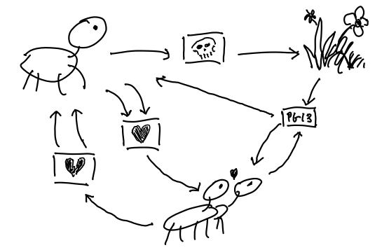
There are some other things about Things that are best expressed outside the Petri Net. For instance, your modelling assumptions that:
- The environment is a closed system:

- Getting together and breaking up happens quickly in comparison to dying and being born, so you consider that subsystem in equilibrium, which also conveniently allows you to express the relative proportion of coupled Things in terms of the whole population of Things, using the Hill equation (see paper for derivation).
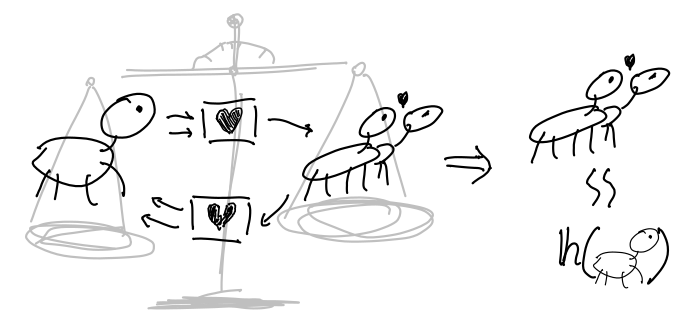
And of course, the underpinning ontological assumption that the Law of Mass Action holds:
Species are valued on a continuum, and the rate at which any process occurs is proportional to the quantities of the input species.
for experts only: it’s a monoid homomorphism from the input leg of the petri net span viewed as a point in the free commutative monoid on species into the multiplication monoid in a polynomial algebra over species that is identity on (individual) species.
So the tower of assumptions looks like this: 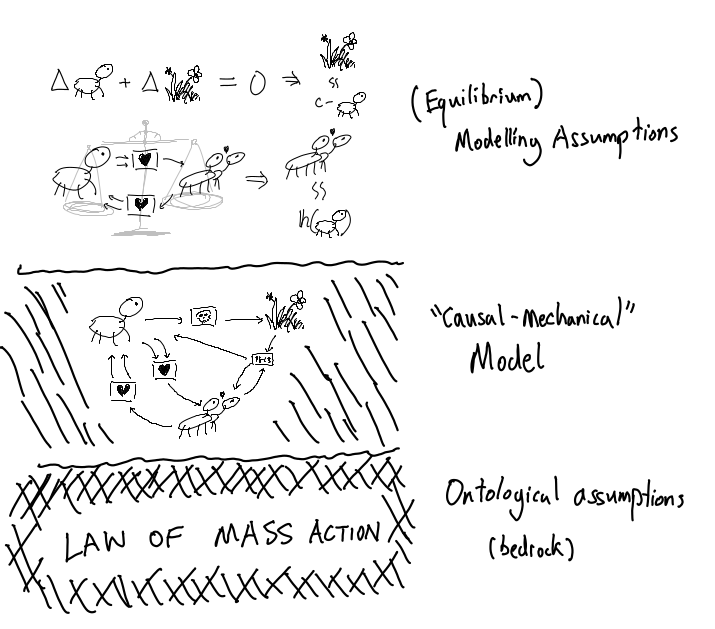
The payoff is an easy way to graphically manipulate Petri Nets to obtain a read-off first-order differential equation. Here’s the procedure:
- Draw Petri Net, where nodes are species, edges have direction and integer multiplicity, and each transition-box is marked with a free variable.
- For each box, multiply the inset variable by the source of each incoming edge.
- For each modelling assumption, perform a variable substitution whereever applicable, and cut all edges going into substituted nodes.
- Cancel opposing pairs of edges, respecting multiplicity.
- For each node, the polynomial defining its rate of change is the sum of all boxes with an edge going into that node (multiplied by multiplicity), minus the sum of all boxes connected by an edge leaving that node.
It looks like this: The first picture is the Petri Net, the second is what happens after step 2, the third what happens after we apply just the closed-system assumption, and the fourth is what happens after we apply all the rest: 
The resulting univariate dynamical system is \(T' := b(c-T)T(\mathbf{h}(T)) - dT\), with free variables \(b,c,d\) and the Hill coefficient of \(\mathbf{h}\). You fit those coefficients to match your observational data of Things, and now you can answer the problematic questions! Model increased birth rate by increasing \(b\), model decreased death rate by decreasing \(d\). The Allee Effect plot at the start of the post was obtained with coefficients \(b \mapsto 0.1, d \mapsto 3.2, c \mapsto 50\), and Hill coefficient \(2\).
I derive a few well-studied univariate dynamical systems in the paper, and show an expressive completeness result: that every F-O ODE in rational functions can be obtained by some Petri Net and some modelling assumptions. But I had the most fun with Hirata et. al.’s study of the HES1 gene regulatory network, which was a real adventure. My good friend who is doing a PhD in biochemistry in Vienna gave me a crash course in gene transcription, and I plumbed some technological extremes: I was measuring off data from printed paper with a ruler to manually transcribe for a gradient descent algorithm!
C. very applied example: HES1 gene regulatory networks
Details about the HES1 gene transcription network are in the paper. Knowing the processes involved, the dynamical system basically writes itself.

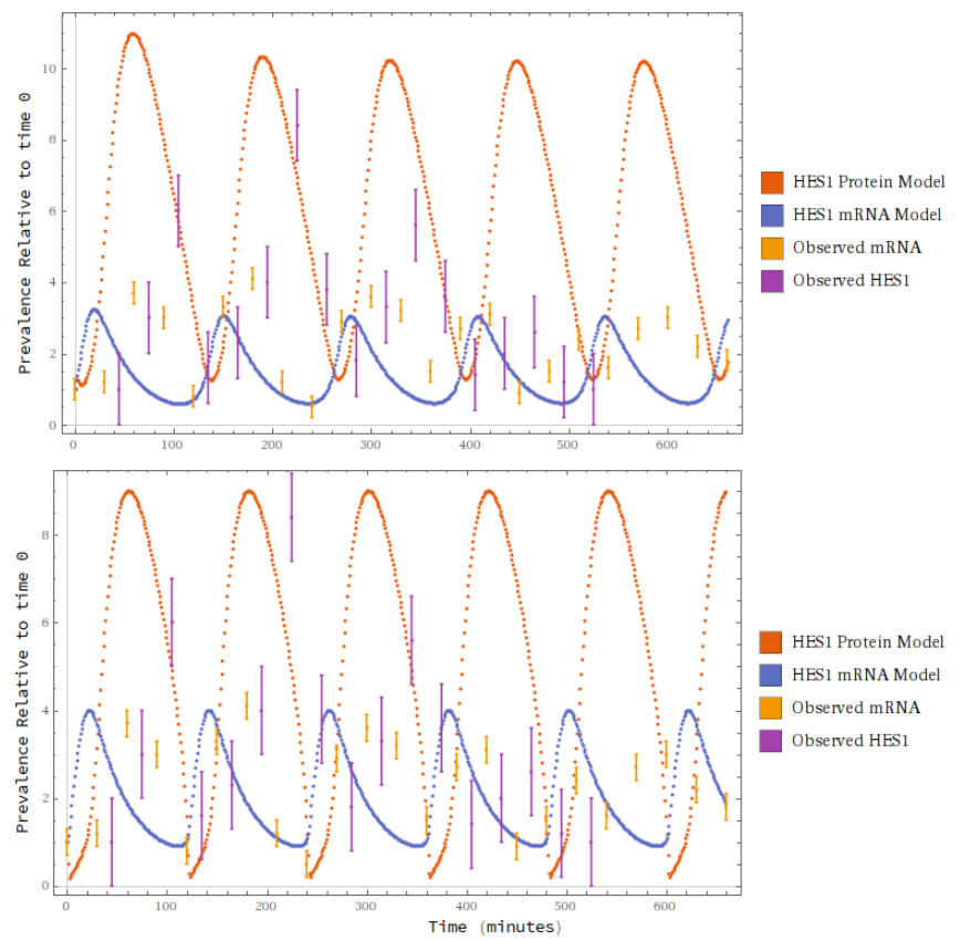
By stochastic gradient descent (and a judiciously chosen loss function) I was able to fit the coefficients of the model against Hirata et al.’s data. It’s not a stellar fit, but it’s qualitatively indistinguishable from Hirata et al.’s own handcrafted F-O ODE model. One of the models below is from a team of biologists, and the other is by some rube. Can you tell which is which?
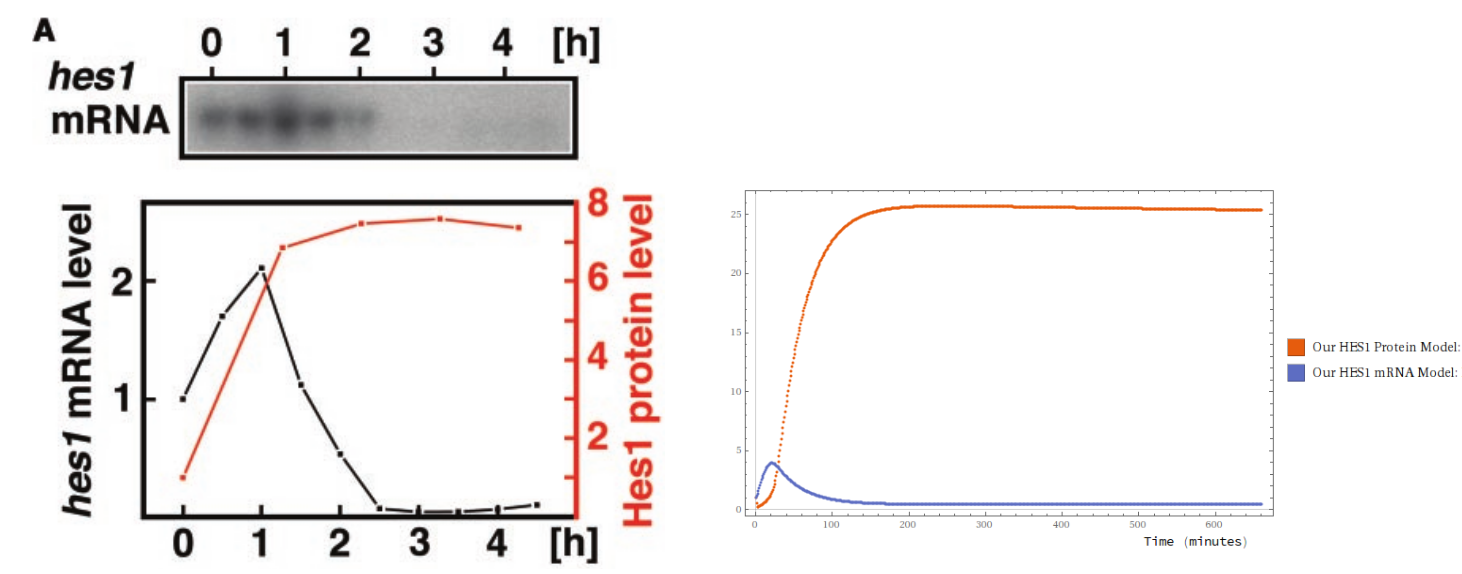
Then I leveraged the information in the Petri Net to do something neat. I tried to predict the effect of a laboratory intervention. This first lab treatment was designed to specifically inhibit a particular transition in the Petri Net. Holding the other coefficients fixed and modulating the targeted coefficient down (to about a hundredth the value), I obtained a qualitative match that exhibited non-periodicity, with exact values within a fair ballpark - less than half an order of magnitude.
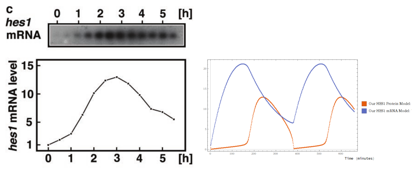
I was able to do the same for both of Hirata et al.’s intervention treatments; the second one below mainly targeted a different process, but had mild effects on others. Again, just modulating down the chiefly targeted coefficient, I got a squint-fit prediction.
This is decent, because the qualitative matches to intervention data are a sniff-test: there’s nothing glaringly wrong about the model at the mechanical level (unsurprising, since the Petri Net was well-informed from the start.) But counterfactually, what would have happened if we started with the wrong mechanism in mind, and so the wrong Petri Net? Of course it could fool our sniff tests on all the interventions we can imagine, but if it fails any sniff test for any intervention, we know the model must be bad.
And that’s what I mean by a scientific method for dynamical systems.